
Prerequisites
For this article, I used a python environment created with Anaconda. The backbone of the environment is Python version 3.7.6 and the analytics were done with Jupiter-notebook. Jupiter-notebook is an interactive web wrapper for Python and other programming languages. The project is hosted here.
Github project structure
├── environment.yml
├── eval_error.py
├── linear_regression.ipynb
├── plotly_linear_model.ipynb
└── README.md
Description
- environment.yml contains the project specifications
- eval_error.py python script calculates the errors
- *.ipynb are two jupyter-notebooks mostly used for graphing
Anaconda environment can be installed with below command:
conda env create -f environment.yml
General Considerations
A Machine-Learning model can be evaluated based on several criteria. These criteria could be related to performance, computational load, or time to converge. But in this article, I will only talk about the most common errors used in Machine-Learning.
The main goal of the analysis is to provide an accurate answer to a particular question. If you think about this a little bit, this is an expression of life itself, it’s beyond the technical domain.
So, let me explain. We begin doing things with a certain belief. We have a World-View, and based on the feedback we adjust our World-View. Maybe something we thought was right, turned out to be completely wrong. Hopefully, we give up bad practices and get good ones.
Bit size philosophy
From a “philosophical point of view”, Machine-Learning is analogous to our World-View. If we receive positive feedback it means that the way we act on the world is correct. If not, we have to change a few things. In a beneficial manner, because it will mean we can grow, we learn.
The general idea is not different when evaluating machine-learning algorithms. We must know how far off was the prediction. What caused the error in our model?
Machine Learning evaluation
The ML process begins by splitting the data into training and testing datasets. The training dataset is made up of features and labels.
These features are the attributes that predict a label or give an outcome.
If we use a real estate for example, the features of a house would be:
- number of rooms
- the year it was built
- the size of the property
The labels are the house prices.
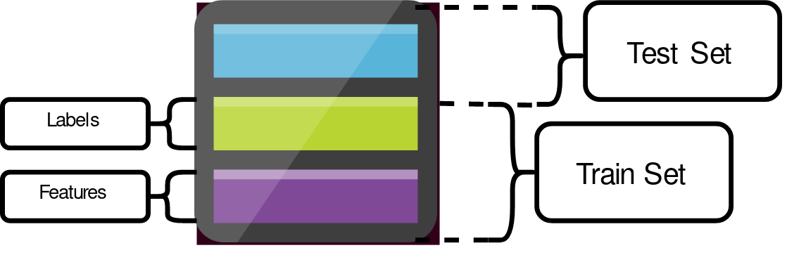
After the training phase, the model is evaluated against the test dataset. This is also known as the evaluation. The differences between the prediction and the actual data tell us how good our model was.
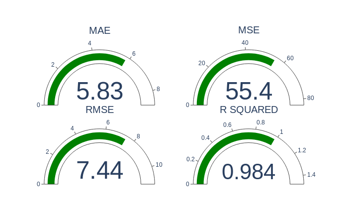
We use errors to score Machine-Learning models.
Some of the most common errors used in Machine-Learning are:
- Mean Absolute Error
- Mean Squared Error
- Root Mean Squared Error
- Root Mean Square Logarithmic Error
- Mean Bias Deviation
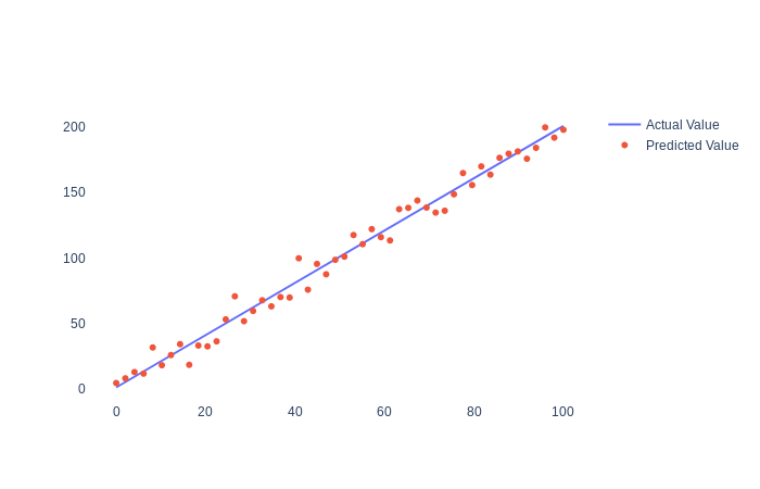
But first, let’s create some synthetic data with python generators:
x = np.linspace(0, 100, 50)
y = 2*x + 1

noise = np.random.normal(0, 7, y.shape)
y_2 = y + noise
The first two lines created a linear equation in 2D space with 50 data point between [0,100]. In the last two lines, we added noise or randomness, so our y coordinates don’t follow a straight line. X coordinates are the same for both samples. y_2 would be in our case the predicted value.
With this small sample, we want to simulate a real case where our model is not perfect. As a side note, we don’t want something that is 100% accurate. This is an indication of overfitting. It means that our model won’t have good results against new data.
The Machine-Learning errors can be calculated with Python or by using Scikit-learn.
Scikit-learn is a scientific library most commonly used in Machine-Learning.
The Machine-Learning errors can be calculated with Python or by using Scikit-learn. Scikit-learn is a scientific library most commonly used in Machine-Learning.
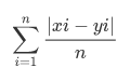
Mean Absolute Error
MAE is the sum of absolute errors divided by the number of samples. Absolute means that we don’t take into account the direction of the error. If xi is the actual value and yi is the predicted one, and data has n samples the MSE can be expressed with this formula:

Python
difference = predict - actual
square_diff = np.square(difference)

score = square_diff.mean()
return score
Scikit-Learn
mae = metrics.mean_absolute_error(y, y_2)
- y the actual value
- y_2 predicted value
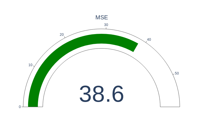
Mean Square Error
MSE is calculated by dividing the corresponding sum of squared errors to the sample size. MSE formula:

- n represents the sample size.
- xi represents the observed values,
- yi the predicted values.
Python
difference = predict - actual
square_diff = np.square(difference)

score = square_diff.mean()
return score
Scikit-Learn
mse = metrics.(y,y_2)
- y the actual value
- y_2 predicted value
MSE is sizable bigger because the errors get raised to the power of two before being averaged.
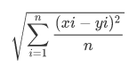
Root Mean Squared Error
RMSE is a quadratic scoring rule that also measures the average magnitude of the error. It’s the square root of the average of squared errors. Here the error represents the difference between prediction and actual value.
RMSE formula:
Python
difference = predict - actual
square_diff = np.square(difference)
mean_square_diff = square_diff.mean()
score = np.sqrt(mean_square_diff)
return score
Scikit-Learn:
rmse = np.sqrt(mse) #mse**(0.5)
The way RMSE is calculated has some implications. The individual errors get exponentiated to two before being averaged. This means the RMSE is much more sensitive to large errors. RMSE is more sensitive to outliers. Outliers are extreme values that deviate from the normal values.
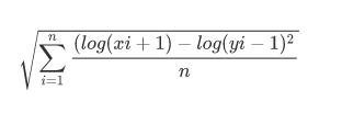
Root Mean Square Logarithmic Error
RMSLE only considers the relative error between the predicted and the actual value. The scale of the error is not important.
RMSLE formula:
MAPE
MAPE is the sum of the individual absolute errors at each moment. It should not be used on low volume data. High level errors during low-demand periods will have a major impact on MAPE.
R Squared
R squared is used to find the optimal parameters in a linear regression model. A linear function is a function whose graph is a straight line on a 2D space. We want to find out what is the least sum of squares to approximate the slope of the function. In the second graph 0.716 represents the slope. By changing slope’s value, we can determine which equation better fits our data.
Linear function:
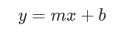
- m is the slope
- b the intersect

Scikit-Learn
r2 = metrics.r2_score(y,y_2)
- y the actual value
- y_2 predicted value
R-squared (R2) measures the dependence of two variables. If we have a variable x and y=f(x), then based on the input x, f(x) should be predictable. If we have a variable x and y=f(x), then based on the input x, f(x) should be predictable.

References:
* https://en.wikipedia.org/wiki/Coefficient_of_determination
* https://blog.minitab.com/blog/adventures-in-statistics-2/regression-analysis-how-do-i-interpret-r-squared-and-assess-the-goodness-of-fit
* https://www.investopedia.com/terms/r/r-squared.asp
* https://medium.com/analytics-vidhya/root-mean-square-log-error-rmse-vs-rmlse-935c6cc1802a
* https://en.wikipedia.org/wiki/Mean_squared_error
* https://en.wikipedia.org/wiki/Mean_absolute_error
* https://docs.conda.io/projects/conda/en/latest/user-guide/tasks/manage-environments.html